3. Matplotlib box plot
Here are the different parts of a box plot and what they represent:
Box: The box represents the interquartile range (IQR), which is the range between the first quartile (Q1) and the third quartile (Q3) of the data. The height of the box is equal to the IQR and represents the middle 50% of the data.
Median line: The median line is drawn inside the box and represents the median value of the data. The median is the middle value when the data is sorted in ascending order. If there is an even number of observations, the median is calculated as the average of the two middle values.
Whiskers: The whiskers extend from the box to the smallest and largest observations that are not considered outliers. The length of the whiskers represents the range of the data within 1.5 times the IQR from Q1 or Q3.
Outliers: Outliers are observations that fall outside 1.5 times the IQR from Q1 or Q3. In a box plot, outliers are plotted as individual points outside the whiskers.
Caps: The caps are horizontal lines drawn at the ends of the whiskers. They represent the smallest and largest observations that are not considered outliers.
3.1. Random box plot
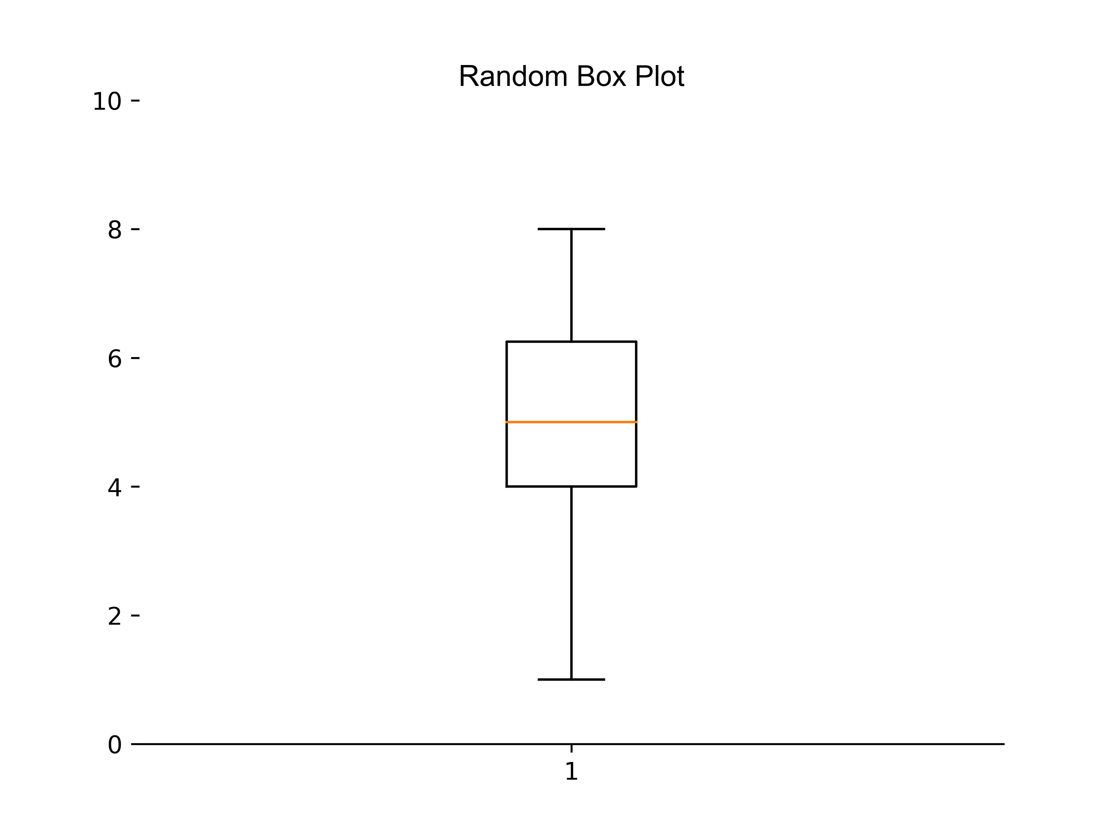
3.2. Python code
 1import numpy as np
 2import matplotlib.pyplot as plt
 3from pathlib import Path
 4
 5
 6def box_plot(data, title):
 7    """
 8    Create a box plot of the given data with the specified title.
 9
10    Parameters:
11    data (array-like): The data to plot.
12    title (str): The title of the plot.
13
14    Returns:
15    None
16    """
17    # Create a new figure with the specified size
18    # plt.figure(figsize=(6, 6))
19    # Plot the data
20    plt.boxplot(data)
21    # Get the current Axes object
22    ax = plt.gca()
23    # Hide the top, right, and left spines of the plot
24    for spine in ["top", "right", "left"]:
25        ax.spines[spine].set_visible(False)
26    # Set the y-axis limits to include all of the data points
27    ax.set_ylim(0, max(data)+ 2)
28    # Add a title to the plot with the specified text and formatting
29    title_str = title.title()
30    ax.set_title(f"{title_str}", fontdict={"fontname": "Arial", "fontsize": 12})
31    # Get the directory of the current file
32    currfile_dir = Path(__file__).parent
33    # Replace spaces in title with underscores to create filename for saving figure
34    filename = title.replace(" ", "_")
35    # build the image file path
36    filepath = currfile_dir / (f"{filename}.png")
37    # Save figure (dpi 300 is good when saving so graph has high resolution)
38    plt.savefig(filepath, dpi=600)
39    # Show the plot on the screen
40    plt.show()
41
42
43def random_data(min, max, n):
44    """
45    Generate an array of n random integers between min and max, inclusive.
46
47    Parameters:
48    min (int): The minimum value of the range to generate random integers from.
49    max (int): The maximum value of the range to generate random integers from.
50    n (int): The number of random integers to generate.
51
52    Returns:
53    numpy.ndarray: An array of n random integers between min and max, inclusive.
54    """
55    # create a random number generator without a fixed seed
56    rng = np.random.default_rng()
57    # generate an array of n random integers between min and max, inclusive
58    data = rng.integers(min, max + 1, size=n)
59    # return the generated data
60    return data
61
62
63def box_random():
64    data = random_data(1, 8, 20)
65    title = "Random box plot"
66    box_plot(data, title)
67
68
69
70# Call the main function if this file is run as a script
71if __name__ == "__main__":
72    box_random()
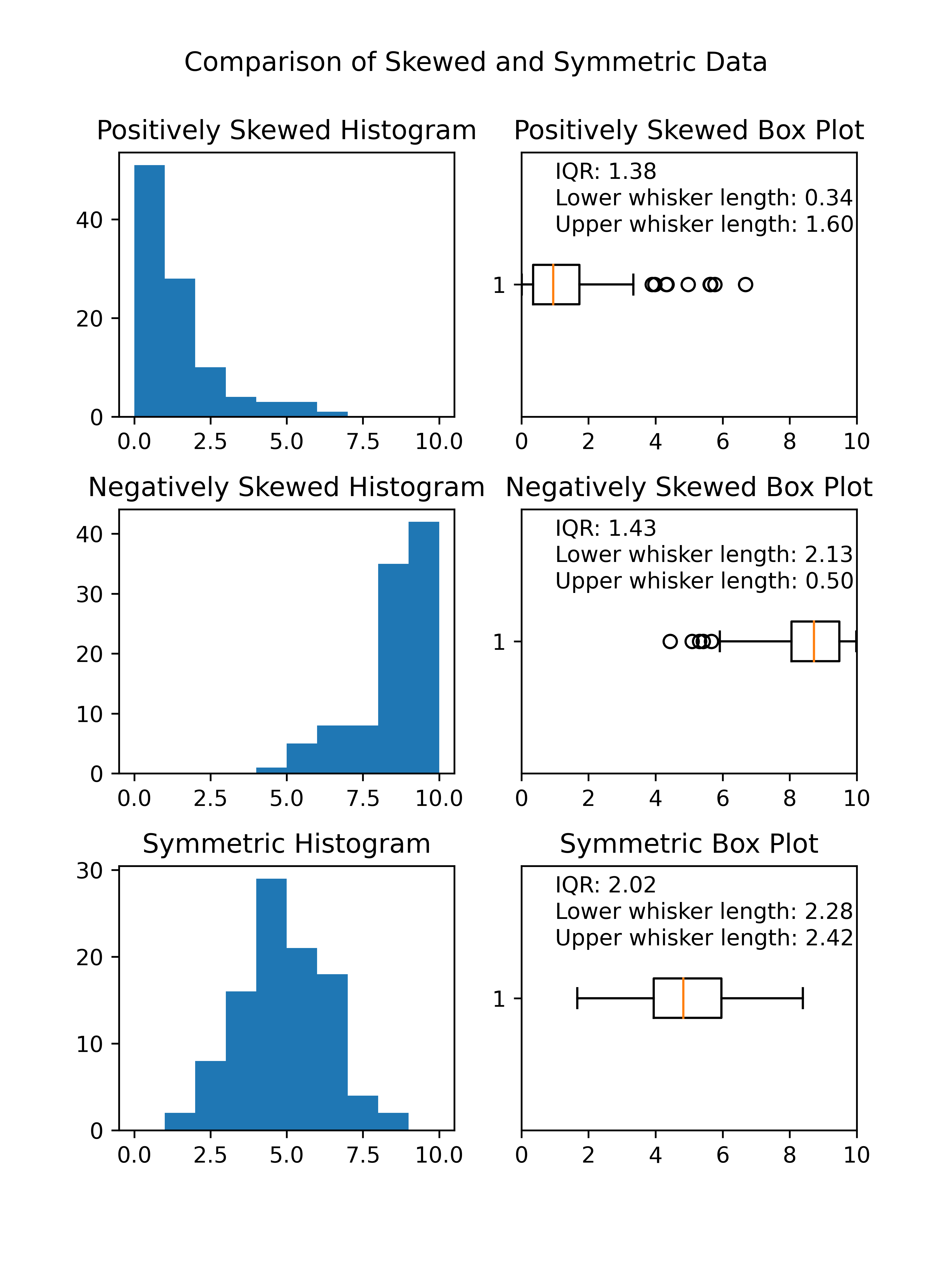
3.3. Comparing skewness in box plots
3.4. Python code
3.5. Version 1 of code
  1import numpy as np
  2import matplotlib.pyplot as plt
  3from pathlib import Path
  4
  5
  6def calculate_boxplot_stats(data):
  7    """
  8    Calculate box plot statistics for a given dataset.
  9
 10    This function takes an array of data as input and returns the interquartile range (IQR),
 11    lower whisker length, and upper whisker length as a tuple.
 12
 13    Args:
 14        data (array-like): An array of data to calculate box plot statistics for.
 15
 16    Returns:
 17        tuple: A tuple containing the IQR, lower whisker length, and upper whisker length.
 18    """
 19    # Calculate the first and third quartiles
 20    q1 = np.percentile(data, 25)
 21    q3 = np.percentile(data, 75)
 22    # Calculate the interquartile range (IQR)
 23    iqr = q3 - q1
 24    # Calculate the lower and upper bounds for outliers
 25    lower_bound = q1 - 1.5 * iqr
 26    upper_bound = q3 + 1.5 * iqr
 27    # Calculate the adjacent values
 28    adjacent_lower = np.min(data[data >= lower_bound])
 29    adjacent_upper = np.max(data[data <= upper_bound])
 30    # Calculate the length of the whiskers
 31    lower_whisker_length = q1 - adjacent_lower
 32    upper_whisker_length = adjacent_upper - q3
 33    return iqr, lower_whisker_length, upper_whisker_length
 34
 35
 36def multi_box_plot():
 37    # Set the random seed for reproducibility
 38    np.random.seed(0)
 39    # Generate positively skewed data
 40    pos_skewed_data = np.random.gamma(shape=1, scale=1.5, size=100)
 41    pos_skewed_data = pos_skewed_data[(pos_skewed_data >= 0) & (pos_skewed_data <= 10)]
 42    # Generate negatively skewed data
 43    neg_skewed_data = 10 - np.random.gamma(shape=1, scale=1.5, size=100)
 44    neg_skewed_data = neg_skewed_data[(neg_skewed_data >= 0) & (neg_skewed_data <= 10)]
 45    # Generate symmetric data
 46    symmetric_data = np.random.normal(loc=5.0, scale=1.5, size=100)
 47    symmetric_data = symmetric_data[(symmetric_data >= 0) & (symmetric_data <= 10)]
 48    # Create figure with 3x2 subplots
 49    fig, axs = plt.subplots(nrows=3, ncols=2, figsize=(6, 8))
 50    fig.subplots_adjust(hspace=0.35)
 51    # Add title to figure
 52    fig.suptitle('Comparison of Skewed and Symmetric Data', y=0.96)
 53
 54    # Create histogram and box plot for positively skewed data
 55    axs[0, 0].hist(pos_skewed_data, bins=10, range=(0, 10))
 56    axs[0, 0].set_title('Positively Skewed Histogram')
 57    axs[0, 1].set_title('Positively Skewed Box Plot')
 58    axs[0, 1].boxplot(pos_skewed_data, vert=False)
 59    axs[0, 1].set_xlim([0, 10])
 60
 61    # Calculate the interquartile range (IQR) and whiskr lengths
 62    iqr, lower_whisker_length, upper_whisker_length = calculate_boxplot_stats(pos_skewed_data)
 63    # Add text labels for box plot statistics
 64    axs[0, 1].text(1, 1.4, f'IQR: {iqr:.2f}')
 65    axs[0, 1].text(1, 1.3, f'Lower whisker length: {lower_whisker_length:.2f}')
 66    axs[0, 1].text(1, 1.2, f'Upper whisker length: {upper_whisker_length:.2f}')
 67
 68    # Create histogram and box plot for symmetric data
 69    axs[1, 0].hist(symmetric_data, bins=10, range=(0, 10))
 70    axs[1, 0].set_title('Symmetric Histogram')
 71    axs[1, 1].set_title('Symmetric Box Plot')
 72    axs[1, 1].boxplot(symmetric_data, vert=False)
 73    axs[1, 1].set_xlim([0, 10])
 74    # Calculate the interquartile range (IQR) and whiskr lengths
 75    iqr, lower_whisker_length, upper_whisker_length = calculate_boxplot_stats(symmetric_data)
 76    # Add text labels for box plot statistics
 77    axs[1, 1].text(1, 1.4, f'IQR: {iqr:.2f}')
 78    axs[1, 1].text(1, 1.3, f'Lower whisker length: {lower_whisker_length:.2f}')
 79    axs[1, 1].text(1, 1.2, f'Upper whisker length: {upper_whisker_length:.2f}')
 80
 81
 82    # Create histogram and box plot for negatively skewed data
 83    axs[2, 0].hist(neg_skewed_data, bins=10, range=(0, 10))
 84    axs[2, 0].set_title('Negatively Skewed Histogram')
 85    axs[2, 1].set_title('Negatively Skewed Box Plot')
 86    axs[2, 1].boxplot(neg_skewed_data, vert=False)
 87    axs[2, 1].set_xlim([0, 10])
 88    # Calculate the interquartile range (IQR) and whiskr lengths
 89    iqr, lower_whisker_length, upper_whisker_length = calculate_boxplot_stats(neg_skewed_data)
 90    # Add text labels for box plot statistics
 91    axs[2, 1].text(1, 1.4, f'IQR: {iqr:.2f}')
 92    axs[2, 1].text(1, 1.3, f'Lower whisker length: {lower_whisker_length:.2f}')
 93    axs[2, 1].text(1, 1.2, f'Upper whisker length: {upper_whisker_length:.2f}')
 94
 95    # Get the directory of the current file
 96    currfile_dir = Path(__file__).parent
 97    # Replace spaces in title with underscores to create filename for saving figure
 98    title = "Skewed and Symmetric Data"
 99    filename = title.replace(" ", "_")
100    # build the image file path
101    filepath = currfile_dir / (f"{filename}.png")
102    # Save figure (dpi 300 is good when saving so graph has high resolution)
103    plt.savefig(filepath, dpi=600)
104    # Show the plot on the screen
105    plt.show()
106
107
108
109# Call the main function if this file is run as a script
110if __name__ == "__main__":
111    # create figure and axes
112    multi_box_plot()
3.6. Version 2 of code
  1import numpy as np
  2import matplotlib.pyplot as plt
  3from pathlib import Path
  4
  5
  6def calculate_boxplot_stats(data):
  7    """
  8    Calculate box plot statistics for a given dataset.
  9
 10    This function takes an array of data as input and returns the interquartile range (IQR),
 11    lower whisker length, and upper whisker length as a tuple.
 12
 13    Args:
 14        data (array-like): An array of data to calculate box plot statistics for.
 15
 16    Returns:
 17        tuple: A tuple containing the IQR, lower whisker length, and upper whisker length.
 18    """
 19    # Calculate the first and third quartiles
 20    q1 = np.percentile(data, 25)
 21    q3 = np.percentile(data, 75)
 22    # Calculate the interquartile range (IQR)
 23    iqr = q3 - q1
 24    # Calculate the lower and upper bounds for outliers
 25    lower_bound = q1 - 1.5 * iqr
 26    upper_bound = q3 + 1.5 * iqr
 27    # Calculate the adjacent values
 28    adjacent_lower = np.min(data[data >= lower_bound])
 29    adjacent_upper = np.max(data[data <= upper_bound])
 30    # Calculate the length of the whiskers
 31    lower_whisker_length = q1 - adjacent_lower
 32    upper_whisker_length = adjacent_upper - q3
 33    return iqr, lower_whisker_length, upper_whisker_length
 34
 35
 36def multi_box_plot():
 37    # Set the random seed for reproducibility
 38    np.random.seed(0)
 39
 40    # Define the properties of each distribution
 41    distributions = [
 42        {
 43            'data': np.random.gamma(shape=1, scale=1.5, size=100),
 44            'hist_title': 'Positively Skewed Histogram',
 45            'box_title': 'Positively Skewed Box Plot'
 46        },
 47        {
 48            'data': 10 - np.random.gamma(shape=1, scale=1.5, size=100),
 49            'hist_title': 'Negatively Skewed Histogram',
 50            'box_title': 'Negatively Skewed Box Plot'
 51        },
 52        {
 53            'data': np.random.normal(loc=5.0, scale=1.5, size=100),
 54            'hist_title': 'Symmetric Histogram',
 55            'box_title': 'Symmetric Box Plot'
 56        }
 57    ]
 58
 59    # Filter the data for each distribution
 60    for dist in distributions:
 61        dist['data'] = dist['data'][(dist['data'] >= 0) & (dist['data'] <= 10)]
 62
 63    # Create figure with 3x2 subplots
 64    fig, axs = plt.subplots(nrows=3, ncols=2, figsize=(6, 8))
 65    fig.subplots_adjust(hspace=0.35)
 66    # Add title to figure
 67    fig.suptitle('Comparison of Skewed and Symmetric Data', y=0.96)
 68
 69    # Create histogram and box plot for each distribution
 70    for i, dist in enumerate(distributions):
 71        axs[i, 0].hist(dist['data'], bins=10, range=(0, 10))
 72        axs[i, 0].set_title(dist['hist_title'])
 73        axs[i, 1].set_title(dist['box_title'])
 74        axs[i, 1].boxplot(dist['data'], vert=False)
 75        axs[i, 1].set_xlim([0, 10])
 76
 77        # Calculate the interquartile range (IQR) and whisker lengths
 78        iqr, lower_whisker_length, upper_whisker_length = calculate_boxplot_stats(dist['data'])
 79        # Add text labels for box plot statistics
 80        axs[i, 1].text(1, 1.4, f'IQR: {iqr:.2f}')
 81        axs[i, 1].text(1, 1.3, f'Lower whisker length: {lower_whisker_length:.2f}')
 82        axs[i, 1].text(1, 1.2, f'Upper whisker length: {upper_whisker_length:.2f}')
 83
 84    # Get the directory of the current file
 85    currfile_dir = Path(__file__).parent
 86    # Replace spaces in title with underscores to create filename for saving figure
 87    title = "Skewed and Symmetric Data"
 88    filename = title.replace(" ", "_")
 89    # build the image file path
 90    filepath = currfile_dir / (f"{filename}.png")
 91    # Save figure (dpi 300 is good when saving so graph has high resolution)
 92    plt.savefig(filepath, dpi=600)
 93    # Show the plot on the screen
 94    plt.show()
 95
 96
 97
 98# Call the main function if this file is run as a script
 99if __name__ == "__main__":
100    # create figure and axes
101    multi_box_plot()