2. Population_sampling
Exploring variation in proportion and means of random samples, drawn from a population
2.1. Population mean
2.2. Sample Mean
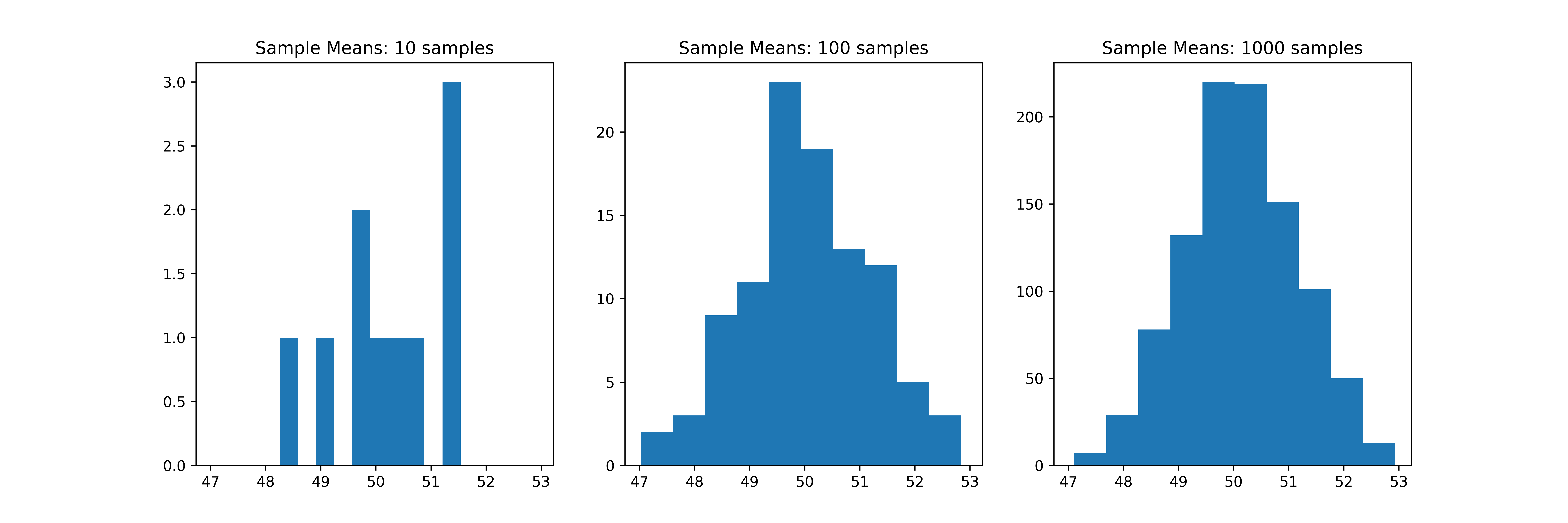
2.3. Sample Means: Increasing samples

 1"""histograms increasing the number of samples
 2"""
 3from pathlib import Path
 4import numpy as np
 5import matplotlib.pyplot as plt
 6
 7currfile_dir = Path(__file__).parent
 8
 9# Set the population parameters
10population_size = 10000
11population_mean = 50
12population_std = 10
13
14# Generate the population
15population = np.random.normal(loc=population_mean, scale=population_std, size=population_size)
16
17# Set the sample parameters
18sample_size = 100
19number_of_samples_list = [10, 100, 1000]
20
21def inc_sample_means(sample_size,number_of_samples_list):
22    fig, ax = plt.subplots(1, 3, figsize=(15, 5), sharex=True)
23    # Generate the samples
24    for i in range(len(number_of_samples_list)):
25        samples = np.random.choice(population, size=(number_of_samples_list[i], sample_size))
26        # Calculate the sample means
27        sample_means = samples.mean(axis=1)
28        # Plot the sample means
29
30        ax[i].hist(sample_means)
31        ax[i].set_title('Sample Means: ' + str(number_of_samples_list[i]) + " samples")
32    # Plot the population histogram
33    # ax[3].hist(population)
34    # ax[3].set_title('Population')
35
36    # Save the figure as a PNG image
37    filepath = currfile_dir / ('sample_means_inc_samples.png')
38    plt.savefig(filepath, dpi=600)
39    plt.show()
40
41inc_sample_means(sample_size,number_of_samples_list)
42
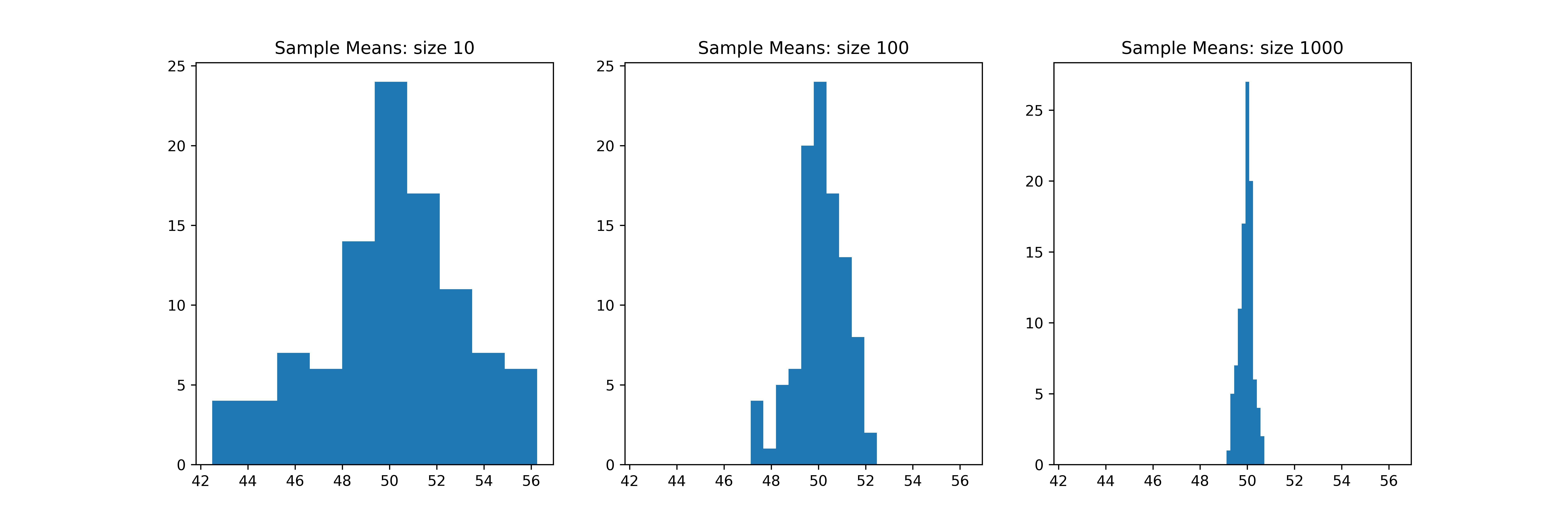
2.4. Sample Means: Increasing sample size

 1"""histograms increasing the sample size
 2"""
 3from pathlib import Path
 4import numpy as np
 5import matplotlib.pyplot as plt
 6
 7currfile_dir = Path(__file__).parent
 8
 9# Set the population parameters
10population_size = 10000
11population_mean = 50
12population_std = 10
13
14# Generate the population
15population = np.random.normal(loc=population_mean, scale=population_std, size=population_size)
16
17# Set the sample parameters
18sample_size_list = [10, 100, 1000]
19number_of_samples = 100
20
21
22def inc_sample_size(sample_size_list,number_of_samples):
23    fig, ax = plt.subplots(1, 3, figsize=(15, 5), sharex=True)
24    # Generate the samples
25    for i in range(len(sample_size_list)):
26        samples = np.random.choice(population, size=(number_of_samples, sample_size_list[i]))
27        # Calculate the sample means
28        sample_means = samples.mean(axis=1)
29        # Plot the sample means
30
31        ax[i].hist(sample_means)
32        ax[i].set_title('Sample Means: size ' + str(sample_size_list[i]))
33    # Plot the population histogram
34    # ax[3].hist(population)
35    # ax[3].set_title('Population')
36
37    # Save the figure as a PNG image
38    filepath = currfile_dir / ('sample_means_inc_size.png')
39    plt.savefig(filepath, dpi=600)
40    plt.show()
41
42inc_sample_size(sample_size_list,number_of_samples)
43
2.5. Population Proportion
2.6. Sample Proportion
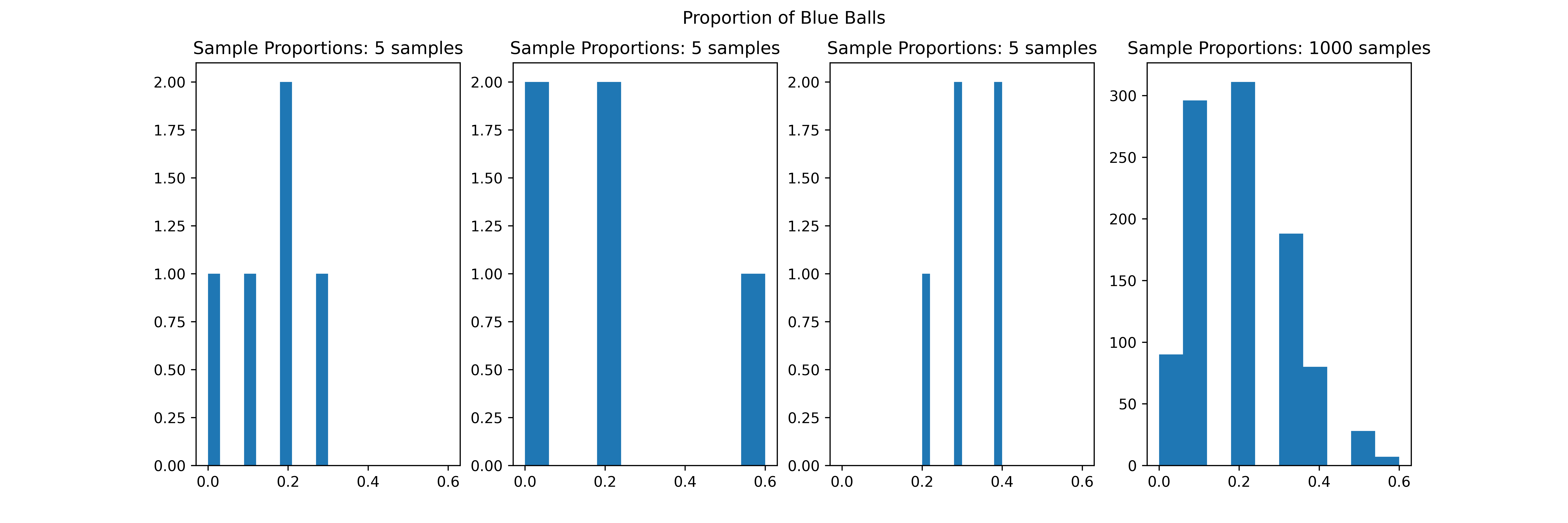
2.7. Sample Proportion: Increasing samples

 1"""histograms increasing the number of samples
 2"""
 3from pathlib import Path
 4import numpy as np
 5import matplotlib.pyplot as plt
 6
 7currfile_dir = Path(__file__).parent
 8
 9# Set the population parameters
10population = ['blue'] * 100 + ['red'] * 400
11
12# Set the sample parameters
13sample_size = 10
14number_of_samples_list = [5, 5, 5, 1000]
15
16def inc_sample_proportions(sample_size,number_of_samples_list):
17    fig, ax = plt.subplots(1, 4, figsize=(15, 5), sharex=True)
18    # Generate the samples
19    for i in range(len(number_of_samples_list)):
20        samples = [np.random.choice(population, size=sample_size, replace=False) for _ in range(number_of_samples_list[i])]
21        # Calculate the sample proportions
22        sample_proportions = [np.mean(sample == 'blue') for sample in samples]
23        # Plot the sample proportions
24
25        ax[i].hist(sample_proportions)
26        ax[i].set_title('Sample Proportions: ' + str(number_of_samples_list[i]) + " samples")
27    # Add a title to the figure
28    fig.suptitle('Proportion of Blue Balls')
29    # Save the figure as a PNG image
30    filepath = currfile_dir / ('sample_proportions_inc_samples.png')
31    plt.savefig(filepath, dpi=600)
32    plt.show()
33
34inc_sample_proportions(sample_size,number_of_samples_list)
35
population = ['blue'] * 100 + ['red'] * 400 creats a population list that contains 500 elements: 100 ‘blue’ strings followed by 400 ‘red’ strings. This represents a population of 500 balls, where 100 are blue and 400 are red.samples = [np.random.choice(population, size=sample_size, replace=False) for _ in range(number_of_samples_list[i])] generates a list of random samples from the population list. Each sample has a size of sample_size and is drawn without replacement.The np.random.choice function is used to generate a single random sample from the population list. The size parameter specifies the size of the sample, and the replace parameter specifies whether sampling should be done without replacement (i.e., whether the same element can be selected multiple times).
The list comprehension [np.random.choice(population, size=sample_size, replace=False) for _ in range(number_of_samples_list[i])] applies this operation number_of_samples_list[i] times to generate a list of number_of_samples_list[i] random samples.
After this line of code is executed, the samples list contains number_of_samples_list[i] random samples from the population list. Each sample is a list of sample_size elements drawn randomly from the population list without replacement.
sample_proportions = [np.mean(sample == 'blue') for sample in samples] calculates the proportion of blue balls in each sample and stores the results in a list named sample_proportions.The expression sample == ‘blue’ creates a Boolean array that has the same shape as sample and contains True where the elements of sample are equal to ‘blue’ and False elsewhere.
The np.mean function calculates the mean of this Boolean array by treating True as 1 and False as 0. This gives the proportion of blue balls in the sample.
The list comprehension [np.mean(sample == ‘blue’) for sample in samples] applies this calculation to each sample in the list samples and stores the results in a new list named sample_proportions.
After this line of code is executed, the sample_proportions list contains the proportion of blue balls in each sample.
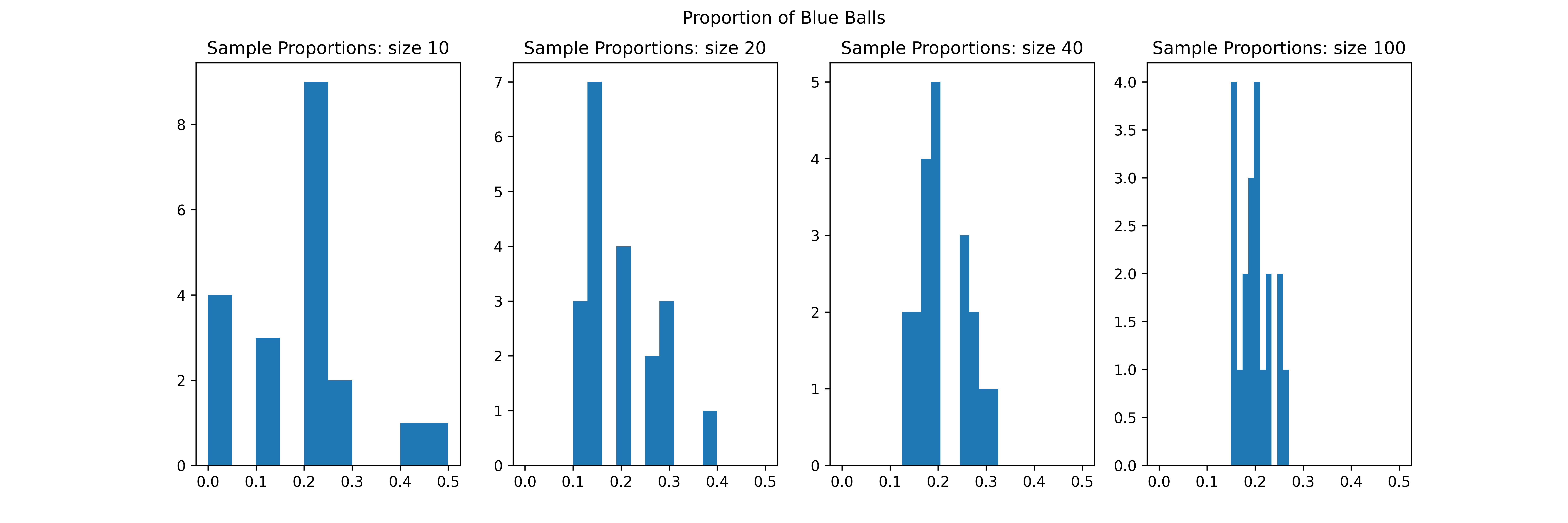
2.8. Sample Proportion: Increasing sample size

 1"""histograms increasing the number of samples
 2"""
 3from pathlib import Path
 4import numpy as np
 5import matplotlib.pyplot as plt
 6
 7currfile_dir = Path(__file__).parent
 8
 9# Set the population parameters
10population = ['blue'] * 100 + ['red'] * 400
11
12# Set the sample parameters
13sample_size_list = [10, 20, 40, 100]
14number_of_samples = 20
15
16def inc_sample_size_proportions(sample_size_list,number_of_samples):
17    fig, ax = plt.subplots(1, 4, figsize=(15, 5), sharex=True)
18    # Generate the samples
19    for i in range(len(sample_size_list)):
20        samples = [np.random.choice(population, size=sample_size_list[i], replace=False) for _ in range(number_of_samples)]
21        # Calculate the sample proportions
22        sample_proportions = [np.mean(sample == 'blue') for sample in samples]
23        # Plot the sample proportions
24
25        ax[i].hist(sample_proportions)
26        ax[i].set_title('Sample Proportions: size ' + str(sample_size_list[i]))
27    # Add a title to the figure
28    fig.suptitle('Proportion of Blue Balls')
29    # Save the figure as a PNG image
30    filepath = currfile_dir / ('sample_proportions_inc_size.png')
31    plt.savefig(filepath, dpi=600)
32    plt.show()
33
34inc_sample_size_proportions(sample_size_list,number_of_samples)
35